Example: Use LSMR algorithm to enhance simulated XRF data

import numpy as np
import matplotlib.pyplot as plt
from PIL import Image

from ptychozoon.vspi_enhance import VSPIFluorescenceEnhancingAlgorithm
from ptychozoon.data_structures import ElementMap, FluorescenceDataset, PtychographyProduct
from ptychozoon.settings import DeconvolutionEnhancementSettings
from ptychozoon.view.vspi_viewer import show_vspi_results

from chronos import plotting as tplot
from chronos.timer_utils import toggle_timer, clear_timer_globals

Generate Data

# width of the probe array in pixels; also determines the distance between
# the edge of the outer edge probe positions and the outer edge of the dummy
# fluorescence array
probe_array_width = 64
# determines the width of the gaussian probe
gaussian_probe_sigma = 7
# approximate number of probe positions; actual count = n_rows * n_cols
n_positions = 30e3

1. Make ptycho array and fluorescence arrays

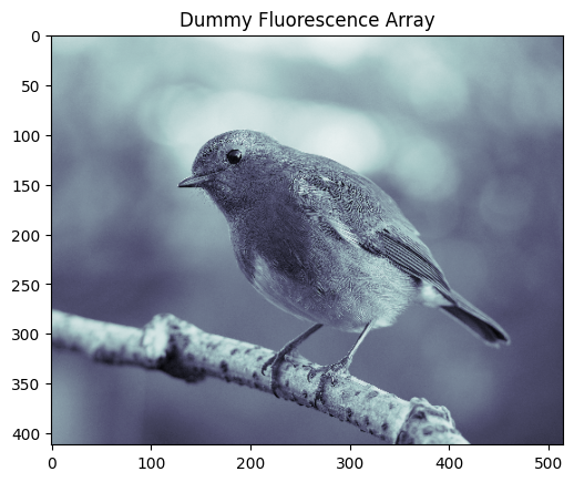
To run this simulation, download the image from this wikipedia link: https://en.wikipedia.org/wiki/European_robin#/media/File:Erithacus_rubecula_with_cocked_head.jpg

img = Image.open("/local/Erithacus_rubecula_with_cocked_head.jpg")   # Load image
s = 5
sample_image = np.array(img).mean(2)[::s, ::s] * 1

plt.title("Dummy Fluorescence Array")
plt.imshow(sample_image, cmap="bone")
plt.show()

object_size = sample_image.shape
element_maps_truth = [ElementMap(name="rubecula", counts_per_second=sample_image)]

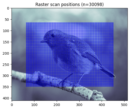
2. Make probe positions

# Raster scan positions covering the area 'padding' pixels from the object edge
padding = probe_array_width
scan_row_min = padding
scan_row_max = object_size[0] - padding
scan_col_min = padding
scan_col_max = object_size[1] - padding

scan_height = scan_row_max - scan_row_min
scan_width  = scan_col_max - scan_col_min

# Grid dimensions that preserve the scan area aspect ratio
aspect = scan_height / scan_width
n_cols = max(1, int(np.round(np.sqrt(n_positions / aspect))))
n_rows = max(1, int(np.round(n_positions / n_cols)))

row_coords = np.linspace(scan_row_min, scan_row_max, n_rows)
col_coords = np.linspace(scan_col_min, scan_col_max, n_cols)

# Raster scan: all rows go left to right
positions = np.array([
    [r, c]
    for r in row_coords
    for c in col_coords
])  # shape: (n_rows * n_cols, 2)  —  axis 0 = row, axis 1 = col (pixels)

print(f"Grid: {n_rows} rows x {n_cols} cols = {len(positions)} positions")

# Visualise scan path overlaid on the object phase
plt.figure()
plt.imshow(element_maps_truth[0].counts_per_second, cmap="bone", origin="upper")
plt.plot(positions[:, 1], positions[:, 0], ".b", lw=0.5, alpha=1, ms=.5)
plt.title(f"Raster scan positions (n={len(positions)})")
plt.show()

Grid: 149 rows x 202 cols = 30098 positions

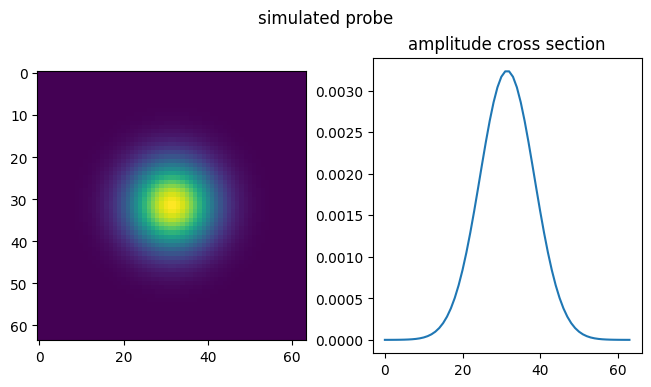
3. Make probe

# Generate complex Gaussian probe
probe_size = (padding, padding)
probe_width = gaussian_probe_sigma
print(f"Probe FWHM: {probe_width * 2 * np.sqrt(2*np.log2(2))}")

# Coordinate grids centred on zero
y = np.linspace(-(probe_size[0] - 1) / 2, (probe_size[0] - 1) / 2, probe_size[0])
x = np.linspace(-(probe_size[1] - 1) / 2, (probe_size[1] - 1) / 2, probe_size[1])
Y, X = np.meshgrid(y, x, indexing="ij")

probe = np.exp(-(X**2 + Y**2) / (2 * probe_width**2)).astype(np.complex128)
probe /= np.sqrt(np.sum(np.abs(probe) ** 2))  # normalise to unit energy
probe /= np.abs(probe).sum()

fig, ax = plt.subplots(1, 2, layout="compressed")
fig.suptitle("simulated probe")
plt.sca(ax[0])
plt.imshow(np.abs(probe))
plt.sca(ax[1])
plt.title("amplitude cross section")
plt.plot(np.abs(probe)[padding // 2])
# plt.axis("off")
plt.show()

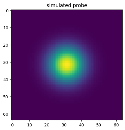
plt.title("simulated probe")
plt.imshow(np.abs(probe))
plt.show()

Probe FWHM: 19.79898987322333

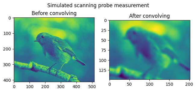
4. Get convolved XRF arrays

i.e. simulate XRF measurement

from scipy.signal import fftconvolve

# Use probe intensity (|probe|^2) as PSF, matching the forward model in enhance.py
probe_intensity = np.abs(probe) ** 2
probe_intensity = probe_intensity / probe_intensity.sum()

# Convolve full object with probe PSF, then sample at scan positions.
# conv_result[r, c] = integral of PSF * element_map_patch centred at (r, c)
element_maps_convolved = []
for element_map in element_maps_truth:
    conv_result = fftconvolve(element_map.counts_per_second, probe_intensity, mode="same")

    # Sample at each scan position (positions are already integer-valued from linspace,
    # but round to be safe)
    pos_idx = np.round(positions).astype(int)
    measurements_flat = conv_result[pos_idx[:, 0], pos_idx[:, 1]]

    # Reshape to (n_rows, n_cols). Raster scan order matches probe_positions order,
    # so this is directly visualizable.
    measurements = np.abs(measurements_flat.reshape(n_rows, n_cols))

    fig, ax = plt.subplots(1, 2, layout="compressed")
    plt.sca(ax[0])
    plt.title("Before convolving")
    plt.imshow(element_map.counts_per_second)#, aspect="auto")
    plt.sca(ax[1])
    plt.title("After convolving")
    ax[1].imshow(measurements)#, aspect="auto")
    plt.suptitle("Simulated scanning probe measurement")
    plt.show()

    element_maps_convolved += [ElementMap(element_map.name, measurements)]

5. Package data into ptychozoon objects

dummy_ptycho_object = np.zeros_like(element_maps_truth[0].counts_per_second, dtype=np.complex128)

# package data
# ptycho
pixel_size_m = 1
probe_positions = positions - np.array(dummy_ptycho_object.shape) / 2
ptycho_in = PtychographyProduct(
    probe_positions=probe_positions,
    probe=probe[None, None],
    object_array=dummy_ptycho_object,
    pixel_size_m=(pixel_size_m,) * 2,
    object_center_m=np.array([0, 0]),
)
# fluorescence
flourescence_in = FluorescenceDataset(element_maps_convolved)

Enhance simulated XRF data

settings = DeconvolutionEnhancementSettings()
settings.solver = "lsmr"
settings.lsmr.max_iter = 100
settings.lsmr.checkpoint_interval = 5
settings.lsmr.damping_factor = 0

# time execution
clear_timer_globals()
toggle_timer(True)

# Create vspi generator 
vspi_runner = VSPIFluorescenceEnhancingAlgorithm().enhance(
    flourescence_in,
    ptycho_in,
    settings=settings,
)

# Run the algorithm
vspi_results = [x for x in vspi_runner]

  0%|                                                                                                                                  | 0/20 [00:00<?, ?it/s]
100%|█████████████████████████████████████████████████████████████████████████████████████████████████████████████████████████| 20/20 [00:20<00:00,  1.03s/it]

%matplotlib qt
viewer = show_vspi_results(vspi_results, block=False)

The previous cell will bring up this GUI:

%matplotlib inline
tplot.plot_elapsed_time_bar_plot_advanced("lsmr", use_long_bar_labels=True);

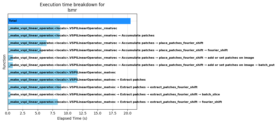
Execution summary of lsmr

Total execution time: 20.5 s

Execution times:
1. _make_vspi_linear_operator.<locals>.VSPILinearOperator._rmatvec: 8.7 s
2. Accumulate patches: 8.7 s
3. place_patches_fourier_shift: 6.5 s
4. fourier_shift: 5.6 s
5. add or set patches on image: 0.83 s
6. batch_put: 0.83 s
7. _make_vspi_linear_operator.<locals>.VSPILinearOperator._matvec: 12 s
8. Extract patches: 12 s
9. extract_patches_fourier_shift: 8.9 s
10. batch_slice: 0.47 s
11. fourier_shift: 8.4 s

Function call stack info:
Ordered by time of first function call
1. _make_vspi_linear_operator.<locals>.VSPILinearOperator._rmatvec
2. _make_vspi_linear_operator.<locals>.VSPILinearOperator._rmatvec → Accumulate patches
3. _make_vspi_linear_operator.<locals>.VSPILinearOperator._rmatvec → Accumulate patches → place_patches_fourier_shift
4. _make_vspi_linear_operator.<locals>.VSPILinearOperator._rmatvec → Accumulate patches → place_patches_fourier_shift → fourier_shift
5. _make_vspi_linear_operator.<locals>.VSPILinearOperator._rmatvec → Accumulate patches → place_patches_fourier_shift → add or set patches on image
6. _make_vspi_linear_operator.<locals>.VSPILinearOperator._rmatvec → Accumulate patches → place_patches_fourier_shift → add or set patches on image → batch_put
7. _make_vspi_linear_operator.<locals>.VSPILinearOperator._matvec
8. _make_vspi_linear_operator.<locals>.VSPILinearOperator._matvec → Extract patches
9. _make_vspi_linear_operator.<locals>.VSPILinearOperator._matvec → Extract patches → extract_patches_fourier_shift
10. _make_vspi_linear_operator.<locals>.VSPILinearOperator._matvec → Extract patches → extract_patches_fourier_shift → batch_slice
11. _make_vspi_linear_operator.<locals>.VSPILinearOperator._matvec → Extract patches → extract_patches_fourier_shift → fourier_shift

from ptychozoon.save import save_vspi_results


save_vspi_results("/local/ptychozoon_test", "results", vspi_results, ".h5", save_every_n_frames=2)

Element arrays saved to /local/ptychozoon_test/results_all_frames.h5